Исследование эпидемиологических данных COVID-19 с использованием вейвлет-анализа

The COVID-19 pandemic has presented an unprecedented global challenge, characterized by a continuous surge of new infections and the emergence of distinct viral variants. The sheer volume and granularity of data collected during this period — encompassing daily case counts, geographical spread, demographic impact, and mortality rates — provide a rich resource for understanding the intricate dynamics of infectious disease transmission

Different viral strains exhibit varied transmissibility, virulence, and immune evasion properties, leading to the manifestation of epidemic processes at diverse scales. Short-term fluctuations might reflect localized outbreaks driven by a highly transmissible variant, while longer-term trends could be influenced by the introduction of new variants, the impact of public health interventions, or seasonal patterns

This is where wavelet analysis

This paper explores the application of wavelet analysis to detailed COVID-19 epidemiological data, demonstrating its efficiency in uncovering intricate patterns and providing a deeper understanding of the multi-scale nature of the pandemic, particularly as influenced by the evolution of its constituent viral strains.

The wavelet transform

The core idea behind the wavelet transform is to decompose a signal into a set of basis functions (wavelets) that are translated and scaled versions of a single “mother wavelet.” The output of the wavelet transform is a set of wavelet coefficients, or a field of continuous wavelet transform field. These coefficients represent the degree of similarity between the signal and the chosen wavelet at a particular scale (inversed frequency) and time location. A large coefficient indicates that the wavelet at that specific scale and time is a good representation of the signal at that point.

Continuous wavelet transform for a given signal

Here

The key advantages of wavelet transform are time-frequency localization, multi-resolution analysis, adaptability for different signal types and successful detection of transient features even for purely-resolved digital sampling.

The wavelet transform is connected with a spectrogram

where

Based on the wavelet transform, wavelet scattering transform (WST)

The WST operates through a series of cascaded layers, each employing a wavelet transform followed by a non-linear operation. This layered structure allows for the progressive capture of increasingly complex signal properties.

At the foundation of the WST lies the zero-order scattering coefficient

The first layer of the WST generates the first-order scattering coefficients (

A key principle underpinning the WST’s ability to capture multi-scale information is the exponential expansion of scales. The wavelet filters are applied at scales that increase exponentially (or according to a geometric progression). This ensures that the decomposition covers a wide range of temporal or spatial resolutions, from very fine details to very coarse structures. This exponential expansion is crucial for capturing the full spectrum of underlying phenomena, from rapid fluctuations to long-term trends, which is particularly relevant when analyzing signals with diverse temporal characteristics, such as epidemiological data influenced by different viral strains operating at different timescales.

Subsequent layers of the WST build upon the information captured in the previous layers. For instance, the second-order scattering coefficients (

As a data, the new cases distributed by the regions of Russia will be used. An example is represented on Figure 1. The data has typical oscillations with a sharp peak in the beginning of 2022 corresponding the Omicron strain appearance.

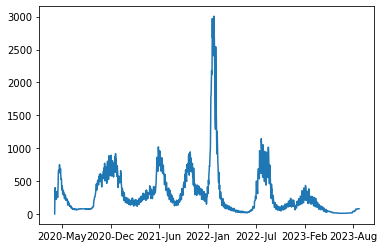
Overall behaviour of new cases in Moscow

example region

DOI:10.60797/BMED.2026.9.7.1

Открыть в полном размереСкачать рисунок

The data considered contains about 1200 counts. Despite the frequent records respectively other epidemiological data, they are not enough for the spectrogram of a good quality (Figure 2). The point is that the spectrogram is represened in "time-frequency" axis; the typical frequencies are respectively low, and the existing amount of data does not allow to resolve the spectrogram efficiently both in frequential and temporal localization. As a result, the spectral lines are heavily enwiden. Spectrogram are proper for more data (which is rare in epidemiology) or in orher fields of science (e.g. physics

[9]

).

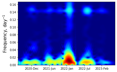
Figure 2 - Spectrogram for Moscow data

DOI:10.60797/BMED.2026.9.7.2

Открыть в полном размереСкачать рисунок

Wavelet scalogram is capable to solve this problem. Despite the maintaining the principle limitation that the diagram cannot be resolved in the both axes, it turns out to be more representative, partially because it is noted in time scales instead of frequencies, partially because the wavelet transform is more robust for abrupt spectral component appearance. On Figure 3, one can see the typical time scales of ~200 days, with the appearance of smaller scales indicating faster processes in the vicinity of Jan 2022 which is connected with Omicron strain. As it can be note, time scales on the wavelet scalogram are more comprehensible than in the spectrogram and visualizes anomalies.

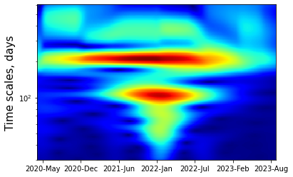
Figure 3 - Wavelet scalogram for Moscow

DOI:10.60797/BMED.2026.9.7.3

Открыть в полном размереСкачать рисунок

To compare the difference in the behaviour in different regions, the wavelet-coherence

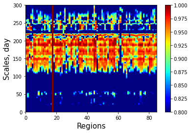
Figure 4 - Wavelet-coherence for Moscow as refercnce region

DOI:10.60797/BMED.2026.9.7.4

Открыть в полном размереСкачать рисунок

As a deeper look, let us consider wavelet scattering transform (WST) made applied to our data. It is a powerful feature extraction technique that generates a hierarchical and invariant representation of signals. Its effectiveness hinges on a set of defining parameters and the specific nature of the coefficients

$S_0$

and

$S_1$

it produces. WST is governed by parameters such as

$J$

representing the total number of scales (or decomposition levels) to be analyzed, and

$Q$

which dictates the number of wavelets used to cover each frequency octave. A larger

$J$

allows for the examination of features across a broader spectrum of resolutions, from fine to coarse, while a higher

$Q$

provides finer discrimination within each frequency band. Together, these parameters define the grid of wavelet filters used, tailoring the analysis to the signal’s expected characteristics and the desired level of feature detail. It should be noted that scales investigated has an exponential expansion.

At the foundation of the WST lies the zero-order scattering coefficient

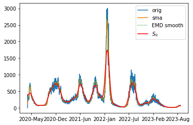
Figure 5 - Illustration of S0 work and different smoothings for Moscow data

DOI:10.60797/BMED.2026.9.7.5

Открыть в полном размереСкачать рисунок

However, building upon

$S_0$

, the first-order scattering coefficients

$S_1$

can be useful for the data's behaviour analysis on the different scales are derived from the initial layer of the WST. For each scale and translation of the wavelet transform applied to the input signal, a set of coefficients is generated. These localized spectral features are then processed through a non-linear function followed by a low-pass filter with a window characteristic for a current scale, a process repeated for all specified scales

$J$

. This cascading approach ensures that the resulting coefficients are largely invariant to translations of the original signal. Each coefficient quantifies the presence and magnitude of a particular spectral characteristic (defined by its scale and translation) across different signal locations, with minimal sensitivity to their exact position. The ensemble of coefficients thus provides a translation-invariant description of the signal’s spectral landscape across various resolutions.

The idea of the application is the following: to compare the local behaviour on the different time scales using

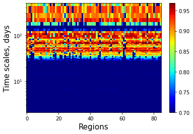
Figure 6 - S1-coherence averaged by reference regions

DOI:10.60797/BMED.2026.9.7.6

Открыть в полном размереСкачать рисунок

For the enhanced interpretability, we also averaged the S1-correlation across all analyzed regions. This process generates a consolidated function that illustrates the overall correlation strength across different time scales (Figure 7). The scales corresponding to the maximum value of this function represent those at which the collective behavior of the regional data is most congruent. This finding has significant implications for prognostic modeling. Specifically, models developed to capture dynamics at these scales of peak correlation are more likely to be generalizable across various geographical areas. In contrast, models focused on shorter time scales, which may capture more localized or transient phenomena, would typically necessitate refitting for each distinct region.

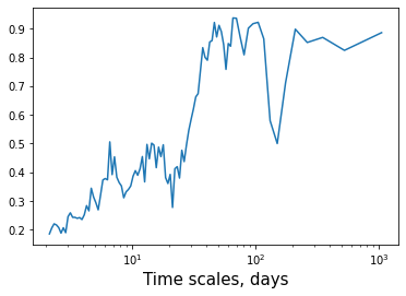
Figure 7 - S1-coherence averaged by reference and target regios

DOI:10.60797/BMED.2026.9.7.7

Открыть в полном размереСкачать рисунок

Having previously discussed anomaly detection in the context of wavelet scalograms, it is appropriate to introduce an additional visualization tool for identifying non-regular behavior. Epidemiological data, when viewed as a complex dynamical system, evolve in a high-dimensional phase space that is inherently difficult to visualize. However, as demonstrated in the preceding analysis, different regions often exhibit similar long-term dynamics, suggesting that the evolution curves of these systems possess identifiable patterns.

To reconstruct the behavior of this multi-component system, we employ Principal Component Analysis (PCA)

Figure 8 illustrates the evolution of new case data for Moscow, with the trajectory colored by time. The Omicron outbreak is clearly visible as a distinct deviation from the primary trajectory (indicated in light green, corresponding to January 2022). Outside of this period, the system exhibits quasi-cyclic behavior, highlighting the stability of the long-term epidemic trends. Note that axes PC1 and PC2 do not have the direct sense because they are the main directions of the PCA which the phase space is projected on. However, it does not interfere the visualisation.

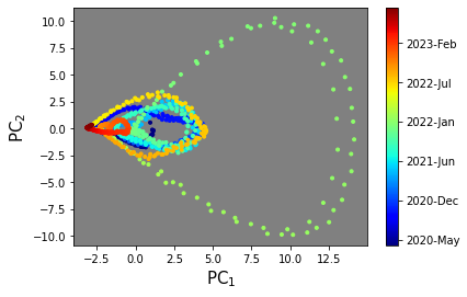
Figure 8 - System behaviour dynamic in Moscow visualization with PCA

DOI:10.60797/BMED.2026.9.7.8

Открыть в полном размереСкачать рисунок

Figure 9 illustrates the overall evolution of the system. The first significant anomaly is observed during the first half of 2021, which coincides with the emergence of the Delta variant. Additionally, the Omicron outbreak is clearly identifiable as a distinct light-green loop in the phase space.

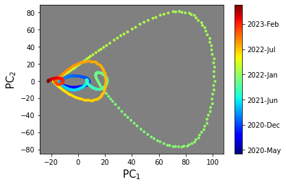
Figure 9 - Overall behaviour dynamic visualization with PCA

DOI:10.60797/BMED.2026.9.7.9

Открыть в полном размереСкачать рисунок

This study successfully leveraged the power of wavelet analysis to unravel the complex, multi-scale dynamics of COVID-19 epidemiological data. By applying wavelet transforms, we were able to decompose the temporal series of infection rates and other relevant metrics into their constituent frequency components, revealing patterns that operate across distinct temporal scales.

A key contribution of this research lies in the application of wavelet coherence analysis. This powerful technique allowed us to not only identify the presence of correlations between different epidemiological signals (e.g., case counts across regions, or case counts and intervention timelines) but also to pinpoint the specific ranges of temporal scales where these correlations are maximized. This finding is crucial, as it suggests that epidemiological processes, driven by factors such as the emergence and spread of specific viral strains, tend to manifest with similar characteristics at certain scales.

The identification of these “privileged” scales of correlation has significant implications for epidemiological modeling and intervention strategies. It suggests that models developed for understanding disease dynamics in one region may indeed be generalizable and transferable to other regions, provided they are applied at these identified scales. This is because the underlying drivers of epidemic spread that are most strongly correlated across different locations appear to operate within these specific frequency bands. Consequently, understanding the dynamics at these particular scales can offer a more robust foundation for predictive modeling and the development of effective public health responses that are less geographically constrained.

Additionally, the PCA projection of the dynamic system is applied and used for the visualization of the system's behaviour. It is shown that it can be successfully used for detection of the anomal behaviour in the data alongside the wavelet transform.